Lecture 8: Motion in Space (Applications of Vector Calculus)
Welcome back! In our lecture on Section 13.2, we learned about the derivatives and integrals of vector functions and how we can view them as velocity and acceleration. In this lecture, we will continue to explore this relationship in much greater detail, combining ideas from sections 13.2 and 13.4 to build a complete toolkit for analyzing how objects move, speed up, slow down, and turn in three-dimensional space.
Topic 1: Velocity, Speed, and Acceleration
We begin by formally defining the key quantities used to describe motion. If $\mathbf{r}(t)$ is the position vector of a particle at time $t$, then its first and second derivatives give us the particle's velocity and acceleration.
Definitions: Velocity, Speed, and Acceleration
- The velocity vector $\mathbf{v}(t)$ is the first derivative of the position vector. It points in the direction of motion and its magnitude is the speed. $$ \mathbf{v}(t) = \mathbf{r}'(t) $$
- The speed v(t) is the magnitude of the velocity vector. It is a scalar quantity. $$ v(t) = |\mathbf{v}(t)| = |\mathbf{r}'(t)| $$
- The acceleration vector $\mathbf{a}(t)$ is the second derivative of the position vector (the derivative of the velocity vector). It describes how the velocity is changing. $$ \mathbf{a}(t) = \mathbf{v}'(t) = \mathbf{r}''(t) $$
Example 1: Chain Rule and Non-Uniform Speed
A particle moves along an elliptical spiral with position function $\mathbf{r}(t) = \langle 10\cos(t^2), 5\sin(t^2), t^2 \rangle$. Find its velocity and acceleration vectors.
A Note on Parameterization:
The projection of this particle's path onto the xy plane is $\langle 10\cos(t^2), 5\sin(t^2), 0 \rangle$. If you plot this in Desmos, you will see that it is an ellipse. However, the space curve 3D path is $\langle 10\cos(t^2), 5\sin(t^2), t^2 \rangle$. The z-component, $z=t^2$, means the particle is also accelerating upwards as it travels. It's helpful to think of it this way: if we let a new parameter be $u = t^2$, then the path could be described by $\mathbf{r}(u) = \langle 10\cos(u), 5\sin(u), u \rangle$. This is a standard elliptical helix. However, since the components of our function are in terms of $t^2$ and not just $t$, the particle does not move along this helix at a uniform rate. The relationship $u=t^2$ means that as $t$ increases, the particle travels along its spiral path faster and faster.
Solution:
We apply the chain rule to each component to find the velocity:
$$ \mathbf{v}(t) = \mathbf{r}'(t) = \langle -10\sin(t^2) \cdot 2t, \ 5\cos(t^2) \cdot 2t, \ 2t \rangle $$ $$ \mathbf{v}(t) = \langle -20t\sin(t^2), 10t\cos(t^2), 2t \rangle $$To find the acceleration, we must use the product rule on the x and y components:
$$ \mathbf{a}(t) = \mathbf{v}'(t) = \langle -20\sin(t^2) - 40t^2\cos(t^2), \ 10\cos(t^2) - 20t^2\sin(t^2), \ 2 \rangle $$Notice that the z-component of acceleration is a constant $2$, so unlike a simple helix, the particle is constantly accelerating upwards.
Use the slider s to see the velocity vector (green) and acceleration vector (purple). Notice they are both changing in magnitude and direction.
Example 2: Product Rule and Finding Velocity at a Point
A particle's position is given by $\mathbf{r}(t) = \langle t\sin(t), e^t\cos(t), \sin(t)\cos(t) \rangle$. Find the parametric equations for its velocity, and then find the velocity vector at the point $(0, 1, 0)$.
Solution:
Step 1: Find the velocity vector $\mathbf{v}(t)$. We use the product rule on each component.
$$ \mathbf{v}(t) = \langle (1)\sin(t) + t\cos(t), \quad e^t\cos(t) - e^t\sin(t), \quad \cos^2(t) - \sin^2(t) \rangle $$The parametric equations for the velocity are:
$$ v_x(t) = \sin(t) + t\cos(t), \quad v_y(t) = e^t(\cos(t) - \sin(t)), \quad v_z(t) = \cos(2t) $$Step 2: Find the value of t that corresponds to the point $(0, 1, 0)$.
To find the velocity at the point $(0,1,0)$, we first need to find the parameter value t that places the particle at that location. We must solve the equation $\mathbf{r}(t) = \langle 0, 1, 0 \rangle$ for t. Once we have the correct value for t, we can substitute it into our velocity function $\mathbf{v}(t)$ to find the velocity at that specific point on the curve.
We set the components of $\mathbf{r}(t)$ equal to the coordinates of the point:
- $x(t) = t\sin(t) = 0 \implies t=0, \pi, 2\pi, \dots$
- $y(t) = e^t\cos(t) = 1$
- $z(t) = \sin(t)\cos(t) = 0$
Let's test $t=0$: $y(0) = e^0\cos(0) = (1)(1)=1$. This matches. $z(0) = \sin(0)\cos(0) = (0)(1)=0$. This also matches. So, the particle is at the point $(0,1,0)$ when $t=0$.
Step 3: Evaluate $\mathbf{v}(t)$ at $t=0$.
$$ \mathbf{v}(0) = \langle \sin(0) + 0\cos(0), e^0(\cos(0)-\sin(0)), \cos(0) \rangle = \langle 0, 1(1-0), 1 \rangle $$The velocity vector at the point $(0,1,0)$ is $\mathbf{v}(0) = \langle 0, 1, 1 \rangle$.
Check Your Understanding
Find the acceleration vector $\mathbf{a}(t)$ for the position function $\mathbf{r}(t) = \langle t^3, e^{2t}, \sin(5t) \rangle$.
Topic 2: Projectile Motion and Integration
If differentiation takes us from position to acceleration, integration allows us to go in reverse. This is the key to solving problems where we know the forces acting on an object (which determine its acceleration) and want to find its path.
Example 3: Finding Velocity and Position from Acceleration
An object has an acceleration vector $\mathbf{a}(t) = \langle 0, 2, 6t \rangle$. Its initial velocity is $\mathbf{v}(0) = \langle 1, 0, 0 \rangle$ and its initial position is $\mathbf{r}(0) = \langle 0, 1, -1 \rangle$. Find its velocity and position vectors.
Solution:
Step 1: Integrate acceleration to find velocity.
$$ \mathbf{v}(t) = \int \mathbf{a}(t) dt = \int \langle 0, 2, 6t \rangle dt = \langle C_1, 2t+C_2, 3t^2+C_3 \rangle $$Use the initial velocity to find the constant vector $\mathbf{C} = \langle C_1, C_2, C_3 \rangle$:
$$ \mathbf{v}(0) = \langle C_1, C_2, C_3 \rangle = \langle 1, 0, 0 \rangle \implies \mathbf{C} = \langle 1,0,0 \rangle $$So, the velocity vector is $\mathbf{v}(t) = \langle 1, 2t, 3t^2 \rangle$.
Step 2: Integrate velocity to find position.
$$ \mathbf{r}(t) = \int \mathbf{v}(t) dt = \int \langle 1, 2t, 3t^2 \rangle dt = \langle t+D_1, t^2+D_2, t^3+D_3 \rangle $$Use the initial position to find the constant vector $\mathbf{D} = \langle D_1, D_2, D_3 \rangle$:
$$ \mathbf{r}(0) = \langle D_1, D_2, D_3 \rangle = \langle 0, 1, -1 \rangle \implies \mathbf{D} = \langle 0,1,-1 \rangle $$Therefore, the position vector is $\mathbf{r}(t) = \langle t, t^2+1, t^3-1 \rangle$.
Example 4: Projectile Motion
A projectile is fired from the origin with an initial speed of $100$ m/s at an angle of $60^\circ$ above the horizontal. Find its position vector $\mathbf{r}(t)$, assuming the only force is gravity (use $g \approx 9.8 \text{ m/s}^2$).
Solution:
Step 1: Start with acceleration. The force of gravity acts downward. If we set up a 2D coordinate system, the acceleration vector is constant:
$$ \mathbf{a}(t) = 0\mathbf{i} - 9.8\mathbf{j} = \langle 0, -9.8 \rangle $$Step 2: Decompose the initial velocity vector into its horizontal and vertical components. We use trigonometry:
$$ \mathbf{v}(0) = \langle 100\cos(60^\circ), 100\sin(60^\circ) \rangle = \langle 100(1/2), 100(\sqrt{3}/2) \rangle = \langle 50, 50\sqrt{3} \rangle $$Step 3: Integrate $\mathbf{a}(t)$ to get $\mathbf{v}(t)$. From Section 13.2, to find $\mathbf{v}(t)$ from $\mathbf{a}(t)$ we can integrate component by component. Remember, the anti-derivative of $0$ is $f(t) = C_1$.
$$ \mathbf{v}(t) = \int \langle 0, -9.8 \rangle dt = \langle C_1, -9.8t + C_2 \rangle $$Using the initial velocity $\mathbf{v}(0) = \langle C_1, C_2 \rangle = \langle 50, 50\sqrt{3} \rangle$, we find $C_1=50$ and $C_2=50\sqrt{3}$. So,
$$ \mathbf{v}(t) = \langle 50, 50\sqrt{3} - 9.8t \rangle $$Step 4: Integrate $\mathbf{v}(t)$ to get $\mathbf{r}(t)$. The initial position is the origin, so $\mathbf{r}(0) = \langle 0,0 \rangle$.
$$ \mathbf{r}(t) = \int \langle 50, 50\sqrt{3} - 9.8t \rangle dt = \langle 50t + D_1, 50\sqrt{3}t - 4.9t^2 + D_2 \rangle $$Using $\mathbf{r}(0) = \langle 0,0 \rangle$, we find $D_1=0$ and $D_2=0$. The final position vector is:
$$ \mathbf{r}(t) = \langle 50t, 50\sqrt{3}t - 4.9t^2 \rangle $$Check Your Understanding
A particle's velocity is given by $\mathbf{v}(t) = \langle t^2, \sin(t), e^t \rangle$. Find its position function $\mathbf{r}(t)$ if the particle starts at the point $\mathbf{r}(0) = \langle 1, 0, 1 \rangle$.
Topic 3: Decomposing Acceleration: The Gas Pedal & Steering Wheel
When an object moves along a curved path, its acceleration vector tells us how its velocity is changing. But this change can be split into two distinct jobs: changing the object's speed and changing its direction. A perfect example is a car entering a freeway on-ramp: it is both turning (changing direction) and speeding up (changing speed). The total acceleration is a combination of the perpendicular "turning" acceleration and the parallel "speeding up" acceleration.
The Two Jobs of Acceleration
- Parallel (Tangential) Acceleration ($a_T$): This part of the acceleration is parallel to the velocity vector. Its only job is to change the object's speed. If it points in the same direction as velocity, the object speeds up. If it points in the opposite direction, the object slows down. Think of this as your gas pedal or your brake.
- Perpendicular (Normal) Acceleration ($a_N$): This part of the acceleration is perpendicular to the velocity vector. Its only job is to change the object's direction, making it turn. This component is what we call centripetal acceleration. It never changes the speed. Think of this as your steering wheel.
Physics Clarification: Centripetal vs. Centrifugal Force
You have likely felt what seems like an "outward" push when turning in a car. This feeling comes from your body's inertia—its desire to continue in a straight line. The real force is the centripetal ("center-seeking") force of the car door pushing you inward to make you turn. The "centrifugal" force is the fictitious or apparent force you feel in response.
| Feature | Centripetal Force | Centrifugal Force |
|---|---|---|
| Direction | Inward, towards the center of rotation | Outward, away from the center of rotation |
| Nature | A real force caused by an interaction (gravity, tension, friction, a car door) | A fictitious or apparent force arising from inertia |
| Frame of Reference | Observed in an inertial (non-accelerating) frame | Experienced in a non-inertial (accelerating) frame |
Summary of Motion Types
- Straight-Line Motion: The direction isn't changing, so the perpendicular (normal) acceleration is zero ($a_N=0$). The entire acceleration is tangential. So if you are driving on a straight road and you push on the gas pedal, all of the acceleration goes to changing the speed of the car.
- Uniform Circular Motion: The speed is constant, but the direction is always changing. The tangential acceleration is zero ($a_T=0$). The entire acceleration is normal, pointing toward the center of the circle. Imagine driving a circular track and you set the cruise control to 30 miles/hr. All of the acceleration is devoted to changing your direction, and none of it is used to change your speed.
- General Curved Motion: Both speed and direction are changing. The object has both tangential ($a_T$) and normal ($a_N$) components of acceleration.
Deriving the Computational Formulas
While the concepts are intuitive, we need practical formulas. We begin by recalling the unit tangent vector, $\mathbf{T}$, which gives the direction of motion. We "normalize" the velocity vector to get a unit vector of length 1:
To save notation, we use an italic v for speed, where $v=|\mathbf{v}|$. This lets us write the velocity vector as the product of its magnitude (speed) and its direction (unit tangent vector):
Now, we differentiate with respect to t. It's crucial to remember that speed, v(t), is a real-valued function of time, not just a number. Therefore, we must use the product rule.
Side Note: Why are $\mathbf{T}$ and $\mathbf{T}'$ Orthogonal?
We know that the magnitude of the unit tangent vector is always 1, so $|\mathbf{T}| = 1$. This implies that $|\mathbf{T}|^2 = 1$, and since the square of the magnitude is the dot product of a vector with itself, we have $\mathbf{T} \cdot \mathbf{T} = 1$. Differentiating both sides of this equation with respect to t gives:
$$ \frac{d}{dt}(\mathbf{T} \cdot \mathbf{T}) = \frac{d}{dt}(1) \implies \mathbf{T}' \cdot \mathbf{T} + \mathbf{T} \cdot \mathbf{T}' = 0 \implies 2(\mathbf{T} \cdot \mathbf{T}') = 0 $$This means $\mathbf{T} \cdot \mathbf{T}' = 0$, which proves they are always orthogonal.
An Intuitive Look: Why Does T' Point "Inward"?
We've proven that $\mathbf{T}'$ is orthogonal to $\mathbf{T}$, but how do we know it points in the direction the curve is turning? Let's think about the definition of the derivative:
$$ \mathbf{T}'(t) = \lim_{h \to 0} \frac{\mathbf{T}(t+h) - \mathbf{T}(t)}{h} $$Imagine two nearby tangent vectors, $\mathbf{T}(t)$ and $\mathbf{T}(t+h)$. The numerator, $\mathbf{T}(t+h) - \mathbf{T}(t)$, is the small vector that represents the change in direction.
Because $\mathbf{T}$ is a unit vector, both $\mathbf{T}(t)$ and $\mathbf{T}(t+h)$ have length 1. If we place them tail-to-tail, their tips lie on a circle of radius 1. As shown in the diagram, the difference vector that connects their tips must point inward, toward the center of the curve's bend. Since $\mathbf{T}'(t)$ points in the same direction as this difference vector, it must also point in the direction of the turn.
Our equation $\mathbf{a} = v'\mathbf{T} + v\mathbf{T}'$ is the heart of the matter. The term $v'\mathbf{T}$ is the tangential component of acceleration, as it's in the direction of motion. The term $v\mathbf{T}'$ is the normal component of acceleration, as it's orthogonal to the direction of motion.
We introduce a new unit vector, the Principal Unit Normal Vector, $\mathbf{N}$, which is defined as the direction of turning: $\mathbf{N} = \frac{\mathbf{T}'}{|\mathbf{T}'|}$. The scalar components are then defined as:
So we can write the full decomposition as:
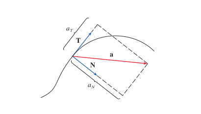
The total acceleration vector, a, is the vector sum of its tangential and normal components.
Deriving the Formula for $a_T$ (The Rate of Change of Speed)
We need a way to calculate $a_T = v' = \frac{d}{dt}|\mathbf{v}|$. We can derive this directly:
$$ v' = \frac{d}{dt}\sqrt{\mathbf{v} \cdot \mathbf{v}} = \frac{1}{2\sqrt{\mathbf{v}\cdot\mathbf{v}}} \frac{d}{dt}(\mathbf{v}\cdot\mathbf{v}) = \frac{1}{2|\mathbf{v}|}(2\mathbf{v}\cdot\mathbf{v}') = \frac{\mathbf{v}\cdot\mathbf{v}'}{|\mathbf{v}|} $$Since $\mathbf{v}' = \mathbf{a}$, this gives our computational formula: $a_T = \frac{\mathbf{v} \cdot \mathbf{a}}{|\mathbf{v}|}$.
Motivation for finding $a_N$: To find a formula for $a_N$, we need a clever way to isolate it. We know that the cross product of any vector with a parallel vector is $\mathbf{0}$. Since $\mathbf{v}$ is parallel to $\mathbf{T}$, if we compute $\mathbf{v} \times \mathbf{a}$, the tangential part will vanish, leaving only the normal part. $$ \mathbf{v} \times \mathbf{a} = \mathbf{v} \times (a_T\mathbf{T} + a_N\mathbf{N}) = a_T(\mathbf{v} \times \mathbf{T}) + a_N(\mathbf{v} \times \mathbf{N}) $$ Since $\mathbf{v}$ and $\mathbf{T}$ are parallel, $\mathbf{v} \times \mathbf{T} = \mathbf{0}$. This leaves $\mathbf{v} \times \mathbf{a} = a_N(\mathbf{v} \times \mathbf{N})$. Taking the magnitude of both sides and using the fact that $|\mathbf{v} \times \mathbf{N}| = |\mathbf{v}||\mathbf{N}|\sin(90^\circ) = |\mathbf{v}|$, we get $|\mathbf{v} \times \mathbf{a}| = a_N|\mathbf{v}|$. Solving for $a_N$ gives our formula.
Computational Formulas for $a_T$ and $a_N$
The derivations lead to these practical formulas. Given a position vector $\mathbf{r}(t)$, let $\mathbf{v}=\mathbf{r}'$ and $\mathbf{a}=\mathbf{r}''$. Then:
$$ a_T = \frac{\mathbf{v} \cdot \mathbf{a}}{|\mathbf{v}|} \quad \text{and} \quad a_N = \frac{|\mathbf{v} \times \mathbf{a}|}{|\mathbf{v}|} $$Example 5: Calculating Components of Acceleration
Find the tangential and normal components of acceleration for the curve $\mathbf{r}(t) = \langle t, t^2, t^3 \rangle$ at $t=1$, and verify that they sum to the total acceleration vector.
Solution:
Step 1: Find velocity and acceleration at t=1.
$$ \mathbf{v}(t) = \langle 1, 2t, 3t^2 \rangle \implies \mathbf{v}(1) = \langle 1, 2, 3 \rangle $$
$$ \mathbf{a}(t) = \langle 0, 2, 6t \rangle \implies \mathbf{a}(1) = \langle 0, 2, 6 \rangle $$
Step 2: Calculate the scalar component $a_T$.
We'll need the dot product and the magnitude of velocity:
- $|\mathbf{v}(1)| = \sqrt{1^2 + 2^2 + 3^2} = \sqrt{14}$
- $\mathbf{v}(1) \cdot \mathbf{a}(1) = (1)(0) + (2)(2) + (3)(6) = 22$
The tangential component of acceleration is:
$$ a_T = \frac{\mathbf{v} \cdot \mathbf{a}}{|\mathbf{v}|} = \frac{22}{\sqrt{14}} $$Step 3: Calculate the component vectors.
First, we need the unit tangent vector $\mathbf{T}(1)$:
$$ \mathbf{T}(1) = \frac{\mathbf{v}(1)}{|\mathbf{v}(1)|} = \frac{\langle 1, 2, 3 \rangle}{\sqrt{14}} $$The tangential vector component of acceleration is $\mathbf{a}_T = a_T\mathbf{T}(1)$:
$$ \mathbf{a}_T = a_T\mathbf{T}(1) = \frac{22}{\sqrt{14}} \left( \frac{\langle 1, 2, 3 \rangle}{\sqrt{14}} \right) = \frac{22}{14} \langle 1, 2, 3 \rangle = \frac{11}{7} \langle 1, 2, 3 \rangle = \left\langle \frac{11}{7}, \frac{22}{7}, \frac{33}{7} \right\rangle $$The normal vector component is found by subtraction: $\mathbf{a}_N = \mathbf{a} - \mathbf{a}_T$.
$$ \mathbf{a}_N = \langle 0, 2, 6 \rangle - \left\langle \frac{11}{7}, \frac{22}{7}, \frac{33}{7} \right\rangle = \left\langle -\frac{11}{7}, \frac{14-22}{7}, \frac{42-33}{7} \right\rangle = \left\langle -\frac{11}{7}, -\frac{8}{7}, \frac{9}{7} \right\rangle $$Step 4: Verification.
Let's add our two component vectors to ensure they reconstruct the original acceleration vector.
$$ \mathbf{a}_T + \mathbf{a}_N = \left\langle \frac{11}{7}, \frac{22}{7}, \frac{33}{7} \right\rangle + \left\langle -\frac{11}{7}, -\frac{8}{7}, \frac{9}{7} \right\rangle = \left\langle 0, \frac{14}{7}, \frac{42}{7} \right\rangle = \langle 0, 2, 6 \rangle $$This matches our original $\mathbf{a}(1)$ exactly. The decomposition works!
Final Practice
Check Your Understanding #1
For the curve $\mathbf{r}(t) = \langle e^t, e^{-t}, \sqrt{2}t \rangle$, find the velocity, acceleration, and speed of a particle at $t=0$.
Check Your Understanding #2
Find the tangential and normal components of acceleration for the helix $\mathbf{r}(t) = \langle \cos t, \sin t, t \rangle$.
Conclusion
Today, we have built a comprehensive toolkit for describing motion in space. We've seen how differentiation reveals velocity and acceleration, and how integration allows us to reconstruct a path from the forces acting upon it. Most importantly, we've learned how to decompose acceleration into its tangential (speed-changing) and normal (direction-changing) components, giving us a much deeper physical insight into how and why an object's trajectory evolves. In our next lecture, we'll shift our focus from the physics of motion to the pure geometry of curves, exploring concepts like arc length and curvature.