Lecture 11: Functions of Several Variables
So far in our study of calculus, we have primarily dealt with two types of functions. The first, from Calculus I, took one real number as input and produced one real number as output, like $y = f(x)$. More recently, we studied vector-valued functions, which take one real number as input and produce a vector as output, like $\mathbf{r}(t) = \langle x(t), y(t), z(t) \rangle$. Now, we shift our perspective to a new and powerful type of function: one that takes multiple real numbers as input and produces a single real number as output.
An analogy might help. A vector function $\mathbf{r}(t)$ can describe the path of a drone flying through a building, where $t$ is time. A function of several variables, however, can describe a property about the room itself, such as the temperature $T(x,y,z)$ at any given point $(x,y,z)$ in the building.
Topic 1: Functions of Two Variables
We'll begin with the simplest case: a function of two variables.
Definition: Function of Two Variables
A function of two variables is a rule that assigns to each ordered pair of real numbers $(x, y)$ in a set $D$ a unique real number denoted by $f(x, y)$.
- The set $D$ is the domain of the function. It is a subset of the $xy$-plane, $\mathbb{R}^2$.
- The set of all possible output values $f(x, y)$ is the range of the function. It is a subset of the real number line, $\mathbb{R}$.
We often write $z = f(x, y)$ to represent the output value.
Example 1: Domain and Range
Find the domain and range of the function $f(x, y) = \sqrt{9 - x^2 - y^2}$.
Solution:
Domain: For the square root to be defined, the expression inside must be non-negative. So, we require $9 - x^2 - y^2 \ge 0$, which can be rewritten as $x^2 + y^2 \le 9$. This is the set of all points $(x,y)$ on and inside a circle of radius 3 centered at the origin. So, the domain is $D = \{(x,y) | x^2+y^2 \le 9\}$.
Range: The output is $z = \sqrt{9 - (x^2+y^2)}$. The smallest possible value of $x^2+y^2$ is 0 (at the origin), giving $z = \sqrt{9} = 3$. The largest possible value of $x^2+y^2$ is 9 (on the boundary of the domain), giving $z = \sqrt{0} = 0$. Since the square root function only outputs non-negative numbers, the range is all values between 0 and 3, inclusive. Range = $[0, 3]$.
The graph of $f(x, y) = \sqrt{9 - x^2 - y^2}$ is an upper hemisphere of radius 3. The domain of this function is the disk in the xy-plane.
Check Your Understanding
Find and sketch the domain of the function $g(x, y) = \ln(y-x^2)$.
Topic 2: Visualizing Functions
We can visualize functions of two variables in several ways. One way is through a table of values. Below is a table for the wind-chill index, $W = f(T, v)$, which is a function of the air temperature $T$ (in °F) and the wind speed $v$ (in mph).
Here, the domain is a set of ordered pairs $(T, v)$. For any given pair, like $(T=35, v=10)$, the table gives us a single output value, $W=27$. This is a discrete representation of the function.
| Temp (°F) | Wind Speed (mph) | ||||||||||
|---|---|---|---|---|---|---|---|---|---|---|---|
| 5 | 10 | 15 | 20 | 25 | 30 | 35 | 40 | 45 | 50 | ||
| 40 | 36 | 34 | 32 | 30 | 29 | 28 | 28 | 27 | 26 | 26 | |
| 35 | 31 | 27 | 25 | 24 | 23 | 22 | 21 | 20 | 19 | 19 | |
| 30 | 25 | 21 | 19 | 17 | 16 | 15 | 14 | 13 | 12 | 12 | |
| 25 | 19 | 15 | 13 | 11 | 9 | 8 | 7 | 6 | 5 | 4 | |
| 20 | 13 | 9 | 6 | 4 | 3 | 1 | 0 | -1 | -2 | -3 | |
A more common and powerful way to visualize these functions is with a graph.
The Desmos graph below plots the 50 discrete points from our wind-chill table. You can imagine that if we had data for every possible temperature and wind speed, these points would merge together to form a continuous surface.
Definition: Graph of a Function of Two Variables
The graph of a function $f$ of two variables is the set of all points $(x, y, z)$ in $\mathbb{R}^3$ such that $z = f(x, y)$ and $(x, y)$ is in the domain of $f$. This graph forms a surface in three-dimensional space.
For example, the graph of a linear function like $f(x, y) = 6 - 3x - 2y$ is a plane. The graph of $f(x, y) = \sqrt{9 - x^2 - y^2}$ is the upper hemisphere of a sphere of radius 3.
Surfaces for $z = 6 - 3x - 2y$ (a plane) and $z = \sqrt{9 - x^2 - y^2}$ (a hemisphere).
Topic 3: Level Curves and Contour Maps
Another excellent way to visualize a surface is to imagine slicing it with horizontal planes. The intersection of the surface with a plane $z=k$ (where $k$ is a constant) creates a curve. The projection of this curve onto the $xy$-plane is called a level curve.
The term "level" implies constancy. In science, we often use the prefix "iso-" (from Greek for "equal") to describe such lines. For example, on a weather map, lines of constant pressure are called isobars, and lines of constant temperature are isotherms. A level curve is an "iso-curve" of a function's graph.
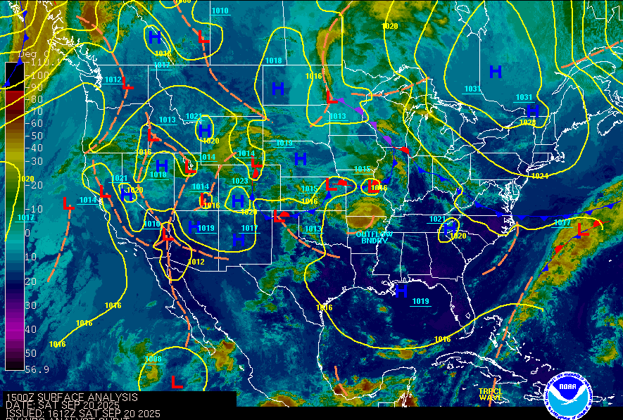
A weather map showing isobars (lines of constant pressure). This is a real-world example of a contour map.
By drawing a collection of level curves for several different values of $k$, we create a contour map. This is exactly what a topographical map is—a 2D representation of a 3D landscape. Where the level curves are close together, the surface is steep. Where they are far apart, the surface is relatively flat. Just as we can create the 2D map by slicing the 3D surface, we can also reconstruct the 3D surface in our minds by "stacking" the 2D level curves at their respective heights ($k$) in space.
Example 2: Finding Level Curves
Sketch the contour map for the function $f(x, y) = x^2 + 4y^2$ using the level curves for $k=1, 4, 9$.
Solution:
The level curves are defined by the equation $f(x, y) = k$.
- For $k=1$: $x^2 + 4y^2 = 1$, which is an ellipse.
- For $k=4$: $x^2 + 4y^2 = 4$, or $\frac{x^2}{4} + y^2 = 1$, a wider ellipse.
- For $k=9$: $x^2 + 4y^2 = 9$, or $\frac{x^2}{9} + \frac{y^2}{9/4} = 1$, an even wider ellipse.
Plotting these ellipses in the $xy$-plane gives us the contour map. The Desmos graph below shows the 3D surface (an elliptic paraboloid) and the level curves being projected onto the $xy$-plane.
Click on the radio buttons on the graph to see the purpose of the contour slices.
Check Your Understanding
The contour map below shows level curves for which type of surface?
a) A plane
b) A cone
c) A paraboloid
Topic 4: Functions of Three or More Variables
We can extend these ideas to functions of three or more variables, like $w = f(x, y, z)$. Here, the domain is a region in $\mathbb{R}^3$. We can no longer visualize the graph, as it would require four dimensions, $(x,y,z,f(x,y,z)) \in \mathbb{R}^4$.
For a function of two variables, the level sets were 2D curves. For a function of three variables, the level sets are 3D level surfaces, defined by the equation $f(x, y, z) = k$.
A perfect analogy is the temperature in this room, $T(x,y,z)$. We can't see the 4D graph of temperature, but we can imagine the 3D surfaces where the temperature is constant. A surface where the temperature is always 70°F is a level surface (an isotherm). Another surface where the temperature is 72°F is a different level surface.
Example 3: Level Surfaces
Describe the level surfaces of the function $f(x, y, z) = x^2 + y^2 + z^2$.
Solution:
The level surfaces are given by the equation $x^2 + y^2 + z^2 = k$ for $k \ge 0$. This is the equation of a sphere of radius $\sqrt{k}$ centered at the origin. So, the level surfaces form a collection of concentric spheres.
The level surfaces of $f(x, y, z) = x^2 + y^2 + z^2$ are concentric spheres.
Check Your Understanding
Describe the level surfaces of the function $g(x, y, z) = x + 2y + 3z$.
Final Practice
Final Practice Problem #1
Find and sketch the domain of the function $f(x,y) = \sqrt{x^2-1} + \ln(4-y^2)$.
Final Practice Problem #2
Sketch the contour map for the function $f(x, y) = y - x^2$ for the k-values $k=-1, 0, 1, 2$.
Conclusion
Today we introduced functions of several variables, which take multiple inputs to produce a single output. We explored how to define their domains and ranges, and how to visualize them using tables, 3D surface graphs, and 2D contour maps made of level curves. We then extended this idea to functions of three variables, whose behavior can be understood by examining their 3D level surfaces. This foundation will be essential as we begin to apply the concepts of calculus—limits, derivatives, and integrals—to this new, multi-dimensional world.